Coming Soon

Stay tuned for more content!

In the meantime, enjoy this cool 4D graphic I made a few years ago for a class I was in…

Visualizing Complex Functions with Domain Coloring

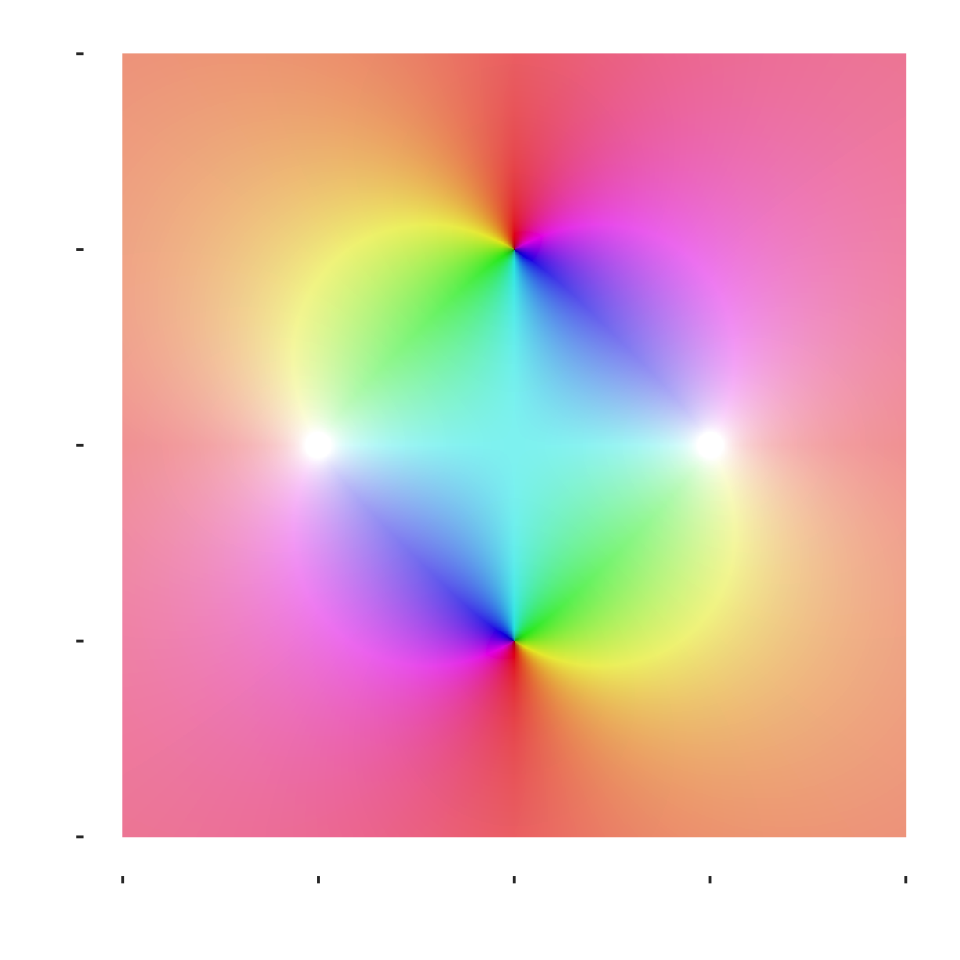
One of the challenges of working with complex-valued functions is that they’re difficult to visualize. For a real-valued function \(f: \mathbb{R} \to \mathbb{R}\), we can easily plot it on a 2D graph. But for a complex function \(f: \mathbb{C} \to \mathbb{C}\), both the input and output are two-dimensional, requiring four dimensions total to represent fully.

Domain coloring provides an elegant solution: we plot the domain (the \(xy\)-plane representing \(\mathbb{C} \cong \mathbb{R}^2\)) and use color to encode information about the output \(f(z)\). Specifically:

• Hue represents the argument (angle) of \(f(z)\): \(\text{Arg}(f(z)) \in (-\pi, \pi]\)
• Lightness represents the modulus (magnitude) of \(f(z)\): \(|f(z)|\)

Below, I’ve visualized the function:

\[f(z) = \frac{z^2 + 1}{z^2 - 1}\]

This function has two roots at \(z = \pm i\) (where the numerator equals zero) and two poles at \(z = \pm 1\) (where the denominator equals zero). In the visualization, you can identify these special points by observing where colors converge or diverge dramatically.

# functions
modulus <- function(z) Re(sqrt(z * Conj(z)))
f <- function(z) (z^2 + 1)/(z^2 - 1)
rad2deg <- function(rad, rotate = 0) ((rad + rotate) * 360/(2*pi)) %% 360

# definitions
# boundaries
L <- -2
U <- 2
# making mesh
domain <- seq(L, U, length.out = 1001)

mesh <- expand.grid(domain, domain) |> 
  mutate("x" = Var1, 
         "y" = Var2) |> 
  select(x, y)

# color mapping components
z <- complex(real = mesh$x, imaginary = mesh$y)

fz <- z |> f()

mod_fz <- fz |> modulus()

# I ended using the second one from the Wikipedia page 
# and I added a constant to shift the color, as well as
# a scale of 100 (a = 0.4 too)

a <- 0.4
ell1 <- (2/pi)*atan(mod_fz) + 65
ell2 <- (mod_fz^a/(mod_fz^a + 1))/10 + 65 
ell3 <- 100*mod_fz^a/(mod_fz^a + 1) + 25 # used this one 

# used saturation of 80
my_colors <- Arg(fz) |>
  rad2deg() |>
  cbind(80, ell3) |> 
  farver::encode_colour(from = "hsl")

df <- cbind(mesh, my_colors) |>
  as.data.frame()

# plot replica attempt
df |>
  ggplot(aes(x, y)) +
  geom_raster(aes(fill = my_colors)) + 
  labs(x = "Re(z)", y = "Im(z)") +
  scale_fill_identity() +
  coord_equal(xlim = c(-2,2), ylim = c(-2,2)) +
  theme(
    panel.background = element_rect(fill = "transparent", color = NA),
    plot.background = element_rect(fill = "transparent", color = NA),
    panel.grid = element_blank(),
    axis.text = element_text(color = "white"),
    axis.title = element_text(color = "white")
  )